Household Energy Assessment

Updated: 3rd July 2021 to use a new tool called SAPjs and discuss our installed air-source heat pump

Perhaps the first step in understanding the energy performance of a house is to carry out a household energy assessment. This page goes through the process I took to create an initial energy assessment for our house before then going on to explore the results.

A little background on assessment tools
Several years ago I worked on a collaboration between OpenEnergyMonitor and CarbonCoop to build an open source energy assessment tool called MyHomeEnergyPlanner. This tool was based on the 2012 version of SAP (Standard Assessment Procedure for UK EPC's (Energy Performance Certificate's) developed by the Building Research Establishment. Carbon Coop are continuing with development of a port of MyHomeEnergyPlanner using Python/Django, renamed Macquette and branded Home Retrofit Planner. Rather than purely an energy assessment tool, Home Retrofit Planner is a much more extensive software application looking at home retrofit in a wholistic way, including all the considerations around measures applied, PAS2035 etc. If this sounds like what you are after, the source code and documentation for Macquette is available here https://gitlab.com/carboncoop/macquette/.

For my own use, I realised I needed something a bit more basic, a tool that focused on the energy assessment part with full input flexibility for the enthusiast householder. I decided to go back to the underlying SAP model used by MyHomeEnergyPlanner and put together a new user interface with this goal in mind. The new tool is called SAPjs.

SAPjs

SAPjs is available free to use as an online tool hosted on the OpenEnergyMonitor website here:

Launch the online tool: OpenEnergyMonitor.org / SAPjs

The tool will open with the example assessment discussed below. Feel free to play around with changing the different inputs to see how it changes the outputs. Click on New to create a new blank assessment. Click on Save to save your project to your computer locally and Open to open a previously saved project. All calculations happen locally in your browser and no data is saved to the OpenEnergyMonitor server.

The source code is all available on GitHub: https://github.com/TrystanLea/SAPjs/

Note on assessment approach

The process I've documented below starts by using input assumptions suggested in the SAP documentation, I then compare the result to my actual energy costs and wider monitoring and finally adjust the inputs to reflect the monitored values.

Measuring up the house

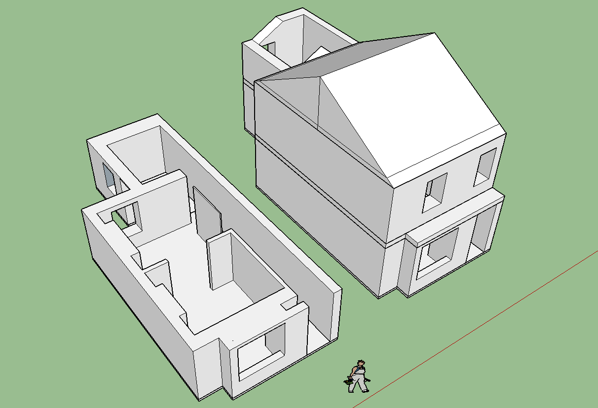
I started by creating a 3D sketchup model of the house so that I could use this model to access any measurements I needed at a later date. In previous assessments that I've done for other buildings I have drawn a 2D floor plan instead which works just as well for the purposes of a basic assessment.

I used a laser measurement tool to take all the measurements.

Here's a screenshot of the resulting sketchup model:

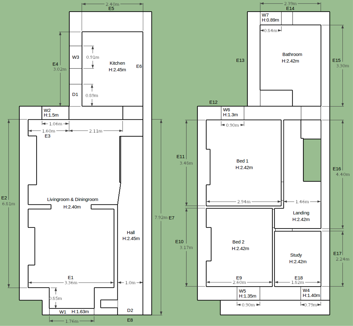
• Measure each wall dimension without initially taking into account the window's and doors, place the dimension on the floor plan.
• Draw an indication of wall width's and include internal walls.
• Draw the windows and doors on the floor plan and note each windows width and height.
• Label each room and note the room height.
• Label each external wall with a unique name: E1, E2, E3 etc
• Do the same for the windows: W1, W2, W3..

Here's my resulting 2D floor plan:

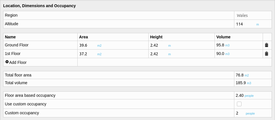
1. Location, Dimensions and Occupancy:

The first section starts with overall building dimensions, noting the floor area and storey heights. The total floor area is calculated by summing up all the room floor areas. I have included the living-room bay window area and slightly longer hall length in my calculation.

For dwelling altitude Google maps is a useful tool.

2. Fabric

The Fabric section is used to enter the dimensions, u-values and other thermal properties of all external and internal walls, floors, the roof and windows of the building.

Walls
Our walls are of stone construction and are plastered on both sides, the thickness varies from 500mm to 800mm with a median of around 550mm.

It is a good idea to spend a bit of time investigating element U-values. This is particularly the case if you have traditional construction, there are many factors that affect the thermal performance of walls from additional layers such as plaster to moisture content.

The Domestic Heating Design Guide v1.0 provides three different U-values for solid stone walls and they are all for unplastered walls:

• Stone 305mm (12in) 2.78 W/K.m2
• Stone 457mm (18in) 2.11 W/K.m2
• Stone 610mm (24in) 1.68 W/K.m2

Historic Scotland performed in-situ monitoring on solid stone walls with the following findings, suggesting generally lower U-values:

• Stone wall 600mm, plaster on laths: 1.1 W/K.m2 +- 0.2W/K.m2
• Stone wall 600mm, drylined with plasterboard: 0.9 W/K.m2 +- 0.2W/K.m2
• Sandstone 550mm, bare: 1.4 W/K.m2 +- 0.1W/K.m2

Although not included in their summary of results a number of walls with plaster on hard where also tested as part of the Historic Scotland study:

• Stone wall 300mm, plaster on hard: 2.3 W/K.m2 (id 1.2)
• Stone wall 350mm, plaster on hard: 1.8 W/K.m2 (id 9.2)
• Stone wall 400mm, plaster on hard: 1.1-1.5 W/K.m2 (id 8.1-4)
• Stone wall 600mm, plaster on hard: 1.6 W/K.m2 (id 1.1)

CIBSE and Energy Savings Trust figures quoted in the Historic Scotland report suggest:

• Energy Savings Trust: 1.7 W/K.m2 for traditional sandstone (or granite) dwelling with solid walls: stone thickness typically 600 mm with internal lath and plaster finish (for the pre‐1919 period)

• CIBSE Guide: 1.38 W/K.m2 for a 600 mm stonewall with a 50 mm airspace and finished with 25 mm dense plaster on laths

The paper 'Solid-wall U-values: heat flux measurements compared with standard assumptions' by the BRI suggests that real world U-values for solid walls may be in the region of 1.3 W/K.m2 rather than 2.1 W/K.m2.

None of the above fit the walls in our house perfectly, as we have an external cement render, a solid stone wall and then plaster on hard, with a total thickness of around 550mm. My guess and starting point will be to model our wall u-values at 1.7 W/K.m2 as this provides a good mid-point between the 350mm and 600mm plaster on hard examples above. It might be a good idea to model a range of U-values from ~1.3 W/K up to 2.1 W/K to understand the implications on total space heating demand.

Floor and Roof
The floor in the living-room has a suspended insulated wooden floor above the underlying solid floor, retrofitted by a previous owner. The total thickness of the insulated floor is 60 mm of which ~20mm is the timber suggesting 40mm of insulation.

The Domestic Heating Design Guide has a number of tables that give U-values for solid floors in contact with earth, depending on the number and lengths of exposed edges.

The main part of the ground floor has two opposite edges exposed at a spacing of about 7m. This would give an insulated U-value of between 0.32 W/K.m2 (50mm insulation) and 0.43 W/K.m2 (25mm insulation). I will use a value in the middle at 0.38 W/K.m2.

The hall has only one edge exposed with a room length of 7m and no insulation suggesting a U-value of 0.38 W/K.m2.

The kitchen has two edges exposed at a combined length of 5.4m and again no insulation suggesting a U-value of 0.9 W/K.m2.

The loft has 250mm of mineral wool insulation, it is however compressed down in places to a minimum of 100mm. The average thickness is more likely in the 200mm range.

CarbonCoop Open Floor U-value calculator
Carbon Coop have also made available an open floor U-value calculator that implements the thermal transmittance calculation of floors as specified in BS EN ISO 13370:2007. With this tool I calculate the U-value of the uninsulated kitchen floor to be 0.994 W/K.m2 and the U-value of the uninsulated hallway floor to be 0.316 W/K.m2 assuming the exposed edge is only the front door opening width of 1m.
http://openflooruvaluecalculator.carbon.coop

Windows
The windows in the house are all double glazed wooden windows but they are all very thin at a spacing thickness of 6mm. Testing for low-E glass coating by checking for a different colour reflection suggests that there is no low-E coating present. Assuming they are air filled rather than argon filled the suggested U-value is ~3.1 W/K.m2.

Both doors contain double glazing, one is otherwise plastic and the other wood. Neither are anything special and so I have assumed for now a U-value of 3.1 W/K.m2 and a frame factor of 0.4 (40% glazed).

SAPjs allows for the definition of the main element types first and then these can be selected when entering each section of wall, floor, roof, windows and doors below it. This arrangement makes it really easy to see the effect of changing the U-values etc on overall heat loss without having to change every element individually.

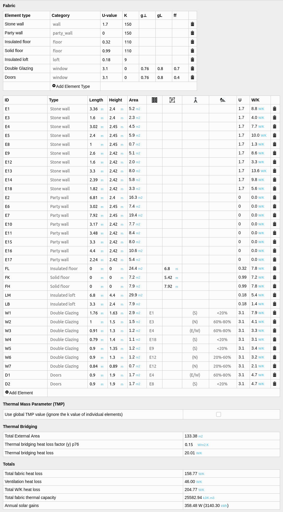
I used the thermal mass parameters of each individual element and entered the default thermal bridging factor of 0.15, all from the SAP documentation.

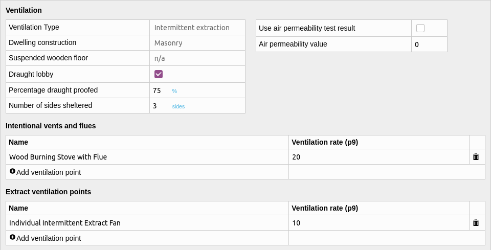
3. Ventilation

The ventilation and infiltration section allows selection of both deliberate ventilation sources and infiltration through the building fabric and other sources of draughts.

Ventilation in our house is achieved by a mixture of open windows when needed and intermittent extract fans. I selected the intermittent extract ventilation option and added two extract fans, one in the kitchen and the other in the bathroom with values as suggested in the SAP documentation.

The house is sheltered to the north and on both sides as it is a terrace house, the front is south facing an relatively unsheltered.

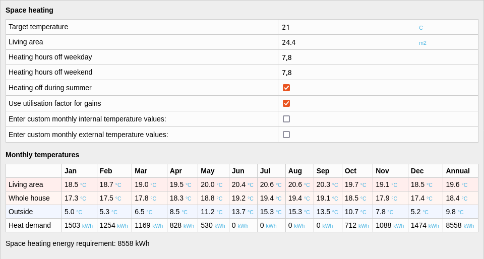
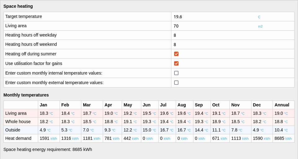
4. Space Heating

The default SAP target temperature is 21C and the default off hours both 7 and 8 hours for weekdays and weekends (p165). This target temperature is higher than our actual target temperature and we usually run the system for longer periods than the default off hours suggest. I will come back to adjust these figures later when I try to match the assessment to my actual monitored values.

I've set the living area initially here to 24.4 m2 the area of the living and dining room, the difference between the living area temperatures and whole house temperatures calculated by SAP suggest that our actual effective living area is larger, I will again come back to adjust this later.

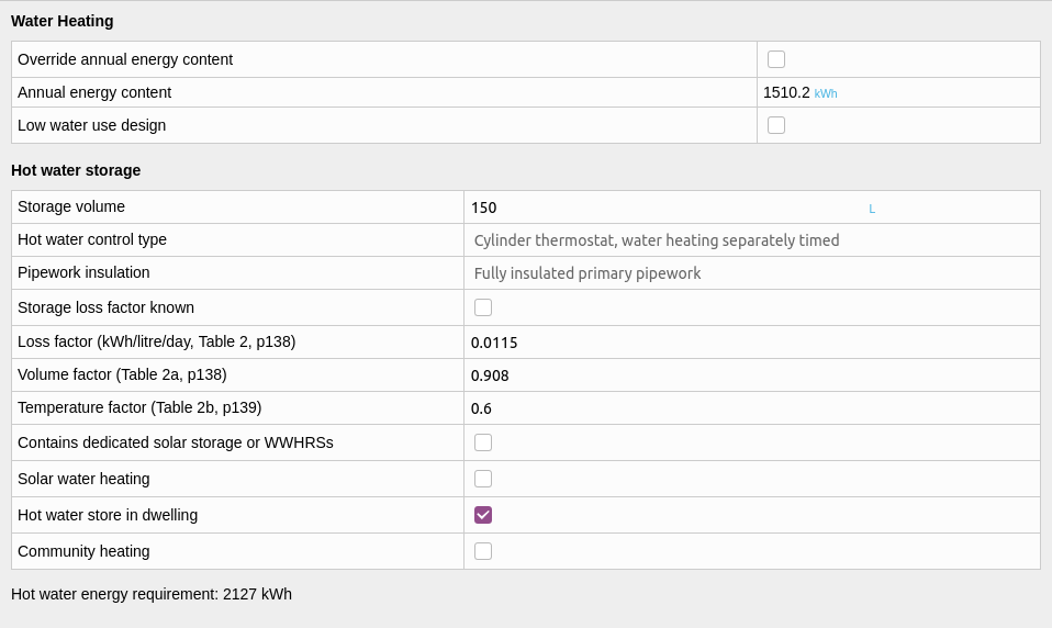
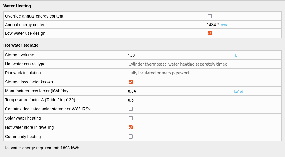
5. Hot water heating

The hot water storage section is shown if a heating system with hot water storage is selected in the heating systems section. We have a 150L cylinder with 75mm of insulation, heated from the heat pump. I've used default values here from the SAP documentation for the loss factor, volume factor and temperature factor.

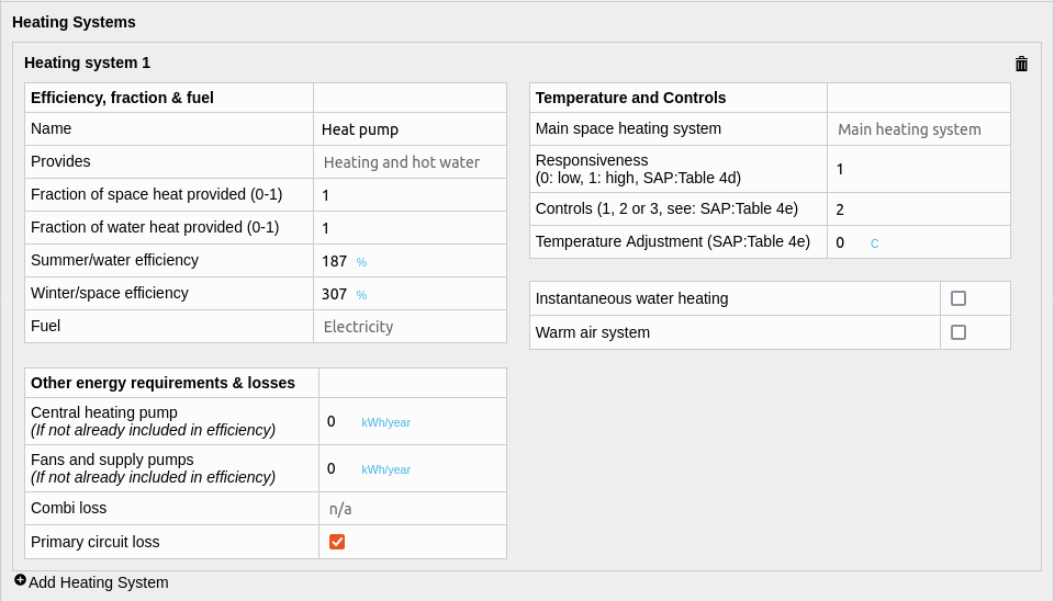
6. Heating Systems

Our heating system is now an air source heat pump. Having monitored the efficiency of the heat pump for over several years, I know it is achieving a combined efficiency of 391% (COP: 3.91).

Ignoring this for now and going by the SAP documentation, the preferred source for efficiency data is the product characteristics database (https://www.ncm-pcdb.org.uk). Unfortunately the efficiency data is not given there in an accessible format but the data files are downloadable and documentation on how to use the data files available from BRE on request. Our 5kW Mitsubushi EcoDan is stated to have a space heating efficiency of 307% at a plant size ratio of 1.0 and a domestic hot water efficiency of 187%.

If heat pump is not listed in the database but has been installed to the MCS standard to work at a flow temperature of <=35C a space heating efficiency of 250% and hot water efficiency of 175% can be assumed. If the system has not been installed to the MCS standard an abysmal efficiency of 170% is to be assumed if you want to follow the SAP documentation to the letter. We can of course enter in our own values here for a more accurate result.

I will start here by entering the figures from the PCDB database and then later look at the difference of using our actual monitored figures.

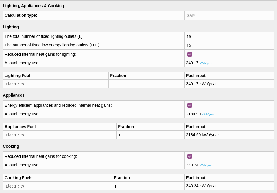
7. Lighting, Appliances & Cooking

Lighting, appliances and cooking all contribute heat gains into a house reducing the amount of heat required from the heating system. It is possible to either use a SAP based calculation as part of this section or a more detailed lighting, cooking and appliance list. Keeping with the approach of starting by using default SAP values I've selected the SAP based calculation to start with.

The SAP calculation suggests a total consumption of 2874 kWh, while our actual consumption was 1584 kWh so quite a bit less!

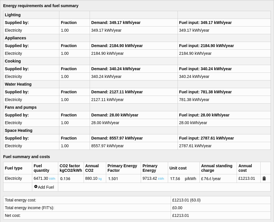
8. Electricity cost, CO2 emissions factor and results

The last section lists all energy and fuel requirements and then calculates the total energy cost, primary energy and CO2 emissions for the dwelling. Using figures from the latest updated version of SAP (SAP 10), the suggested standard electricity tariff rate is 17.56 p/kWh, co2 emissions factor 0.136 kgCO2/kWh and primary energy factor 1.501.

This gives me a total energy cost of £1213/year and CO2 emissions of 880 kg/year.
The rating based on the calculated cost is 63 which corresponds to the rating band D, not great!

9. Comparison with actual energy consumption and costs

The first thing I can do at this stage is compare the calculated energy consumption and costs with my monitored figures. The following table gives a comparison for the last three years, including an projection for 2021.

	SAP	2019	2020	2021
Lighting, appliances and cooing (kWh)	2874	1483	1571	1586
Fans, pumps & heat pump standby	28	0	95	119
DHW Electric (kWh)	781	372	426	479
DHW Heat (kWh)	2127	548	1630	1927
Space Electric (kWh)	2788	1276	1425	1776
Space Heat (kWh)	8558	5047	5986	7506
Total Electric (kWh)	6471	3131	3517	3960
Tariff name	Standard	Ecotricity Fixed	Octopus Agile	Octopus Agile
Tariff unit cost (p/kWh)	17.56	18.86	10.9	~17.5
Total Cost (£)	£1213	£667	£460	£770

Total costs all include a standing charge ~£77/year and I've removed our EV electric use to make the monitored figures comparable.

First we can see that our actual energy costs and consumption are about half the amount suggested by the SAP calculation. There are a lot of changing factors in here, our electricity use appears to have been going up year on year and our unit rate costs have changed quite a bit as well.

We spent less time in the house in 2019, due to both of us spending more time out of the house in our places of work. 2020 changed that of course, both with the pandemic and having a baby. Spending more time in the house meant that the heat pump was left on for longer and average internal temperatures and energy consumption were higher. 2021 has been much the same so far but with the added effect of a prolonged colder winter. Electricity prices have also increased significantly this year and we see the effect of this immediately on the Octopus Agile electricity tariff that we are on.

Still, the SAP figure for total electricity consumption is significantly higher than my range of actual energy consumption and cost figures and so the next step is to look back through the assumptions made in the model to see if we can narrow the gap.

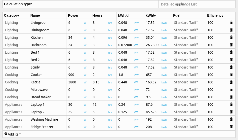
10. Adjusting the assessment to be closer to monitored results

1. The standard lighting, appliances and cooking calculator in the SAP model suggested a consumption of 2874 kWh, almost twice the amount we actually used. An alternative calculation approach is included in the tool called the detailed appliance list, this can be used to match monitored consumption as I have done below, reducing the lighting, appliances and cooking consumption in the model to 1584 kWh.

2. Hot water consumption in the SAP model is not far off my 2021 hot water consumption projection, though it is a fair bit higher than 2020s figure. Selecting low water use design and entering the storage loss factor of our cylinder reduces demand a little to 1893 kWh:

3. Internal temperature. Our actual whole-house internal temperature average for 2020 was 18.7C, higher than the 18.3C predicted by SAP based on the 21C temperature target, living area and occupancy patterns assumed by the SAP calculation. Our winter time whole house temperatures in particular are higher. The difference between the living area temperature and whole house temperature are also smaller.

Increasing the living area to encompass a greater proportion of the house 70m2 instead of 24.4 m2 gives better results for winter temperatures but the average temperature is now a fair bit higher due to predicted higher summer time temperatures.

Reducing the number of weekday off hours to a single 8 hour period and reducing the target temperature to 19.6C seems to give predicted temperatures that are closer to monitored temperatures as it reduces summer temperatures whilst keeping winter temperatures higher. This does however increase predicted space heating demand to 9654 kWh rather than reducing it as we need to match monitored data.

Outside temperatures in 2020 were higher than those used by SAP, our temperatures were closer to those given for the Severn Wales region further to the south of here. Selecting this region reduces the space heating demand back down, near to the original value predicted with the earlier internal temperature assumptions.

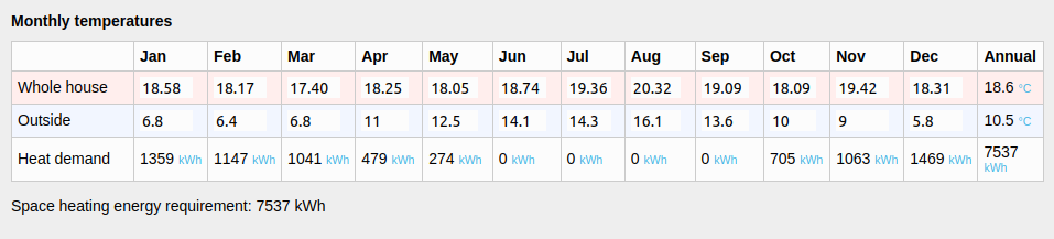
Alternatively it is possible to enter measured internal and external temperatures in the SAPjs interface, doing this drops the space heating energy requirement to 8230 kWh with wind factors based on selecting Wales as the region or 7537 kWh based on selecting Severn Wales. The wind factors here seem to be having more effect! There is a slight difference in solar gain as well but only a few watts.

4. Building fabric and ventilation: At this point our SAP space heating energy requirement is still between 1530 kWh and 2223 kWh greater than our actual metered space heating input in 2020. There are a couple of factors that could account for the remaining difference:

• Over-estimated monitored internal temperatures due to greater temperature differences within the rooms being monitored (E.g colder air temps near external walls than in the middle of the rooms)
• Under estimated building fabric performance
• Lower ventilation losses
• Higher solar irradiation and lower wind speeds than assumed in the SAP dataset
• Higher heat gains from neighbouring houses

Historic Scotland's in-situ monitoring of solid stone walls with plaster on hard had U-values that ranged from 1.1 W/K.m2 to 2.3 W/K.m2. Entering a U-value of 1.1 W/K.m2 in the SAP model reduces space heating demand from 7537 kWh to 6107 kWh, not far off..

Alternatively we could ask how much lower average internal temperature would need to give the same heating demand figure, reducing the average internal temperature by 1C would reduce space heating energy requirement from 7537 kWh to 6458 kWh. The error in internal temperature measurement would need to be ~1.5C to match..

It's perhaps more likely that the difference is due to a combination of factors, one combination could be:

• Custom internal and external temperatures from monitoring
• Wall U-values: 1.4 W/K.m2
• Window U-values: 2.3 W/K.m2 and slightly larger frame factor of 0.8
• Half the ventilation rate for the stove flue (10).

Running these changes through the model gives good agreement with measurements:

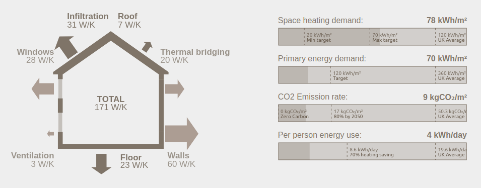
• Heat loss factor of 171 W/K
• Space heating demand 6007 kWh (2020 temperatures, 6009 kWh measured)
• Space heating demand 5283 kWh (2019 temperatures, 5287 kWh measured)

But it is of course hard to say if these are the correct factors to change!

5. Monitored heat pump efficiencies
With the above changes total electricity consumption has reduced from 6471 kWh to 4297 kWh (using 2020 data) but is still a 22% above the measured electricity consumption of 3517 kWh.

Most of this difference is down to the lower assumed heat pump performance of 187% for water heating and 307% for space heating. Entering the actual metered performance of 383% for water heating and 420% for space heating reduces total electricity consumption to 3600 kWh, only 2% above measured 2020 consumption, close enough!

6. Costs
The total energy cost is now £708. To match 2020 costs I just need to enter the 2020 unit rate of 10.9 p/kWh and the cost reduces to £469 which is 2% higher not 260% higher! A similarly close match can be achieved for 2019 and projected 2021 figures with the correct unit rates, heating demand and heat pump efficiencies relating to those years.

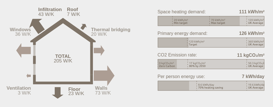
Here's the final headline graphic produced by SAPjs for our house:

11. Predicting savings through building fabric improvement

With the model calibrated it's now relatively easy to explore different ideas for improving building fabric performance and how much these measures might save financially. Here are a couple of initial examples. Assumed electricity cost: 17.5 p/kWh

120mm external wall insulation (0.273 W/K.m2):
Electricity cost of £599/year down from £706/year, a saving of £107/year.

High performance windows (0.85 W.K/m2):
Electricity costs of £678/year down from £706/year, a saving of £28/year.

These are clearly going to take a long time to pay back given the likely costs of these measures.

Reflections

My initial assessment created using a combination of standard SAP input assumptions and my rough research on suitable U-values estimated our energy consumption to be almost double our actual monitored energy consumption. This goes to show how large a difference there can be! Had I calculated payback times of energy efficiency measures based on these initial figures without a cross checking process with actual consumption data, there would have been a significant error!

By using the data I had collected through detailed monitoring I was able to adjust a good portion of the input assumptions in order to bring them closer but I also had to guess as to several other factors that might add up to my lower actual energy consumption.

All in all, I think the key benefit I get from the process is a more in depth understanding of all of the different factors that contribute to the energy performance of our house and at least a rough idea of how the different fabric elements of the house contribute to heat loss and space heating demand.

With the model calibrated I can get a better idea of the kind of savings I might expect from different fabric improvements which is really useful!