Modelling heat transfer in 2D with Agros2D

Building energy modelling tools such as SAP & PHPP are simplified 1D, steady-state models. The thermal model of a building in a 1D model is made up of a list of independent elements: walls, floors, windows etc where heat loss through each element is calculated in 1D perpendicular to the plane of the element.

SAP uses internal element dimensions to define the building envelope, if you imagine two walls coming together at a corner there is a volume of material contained in the corner through which heat loss occurs that is therefore not taken into account.

You could also imagine externally insulating one wall of a stone house where the ends of the wall are still exposed. Heat will still be lost out of that externally insulated wall section through these exposed ends of the wall - but a basic 1D calculation cant really take into account these details and will instead model the wall as a perfectly insulated external wall section.

I've wanted to get a better grasp of how significant the difference might be between a more complete model of the geometry and the simplified 1D approach and am aware from the work of others that models capable of 2D heat transfer are often used for this kind of simulation. The screenshots produced are often quite beautiful with the colour shading showing the heat transfer through the complex geometry of a say a window frame.

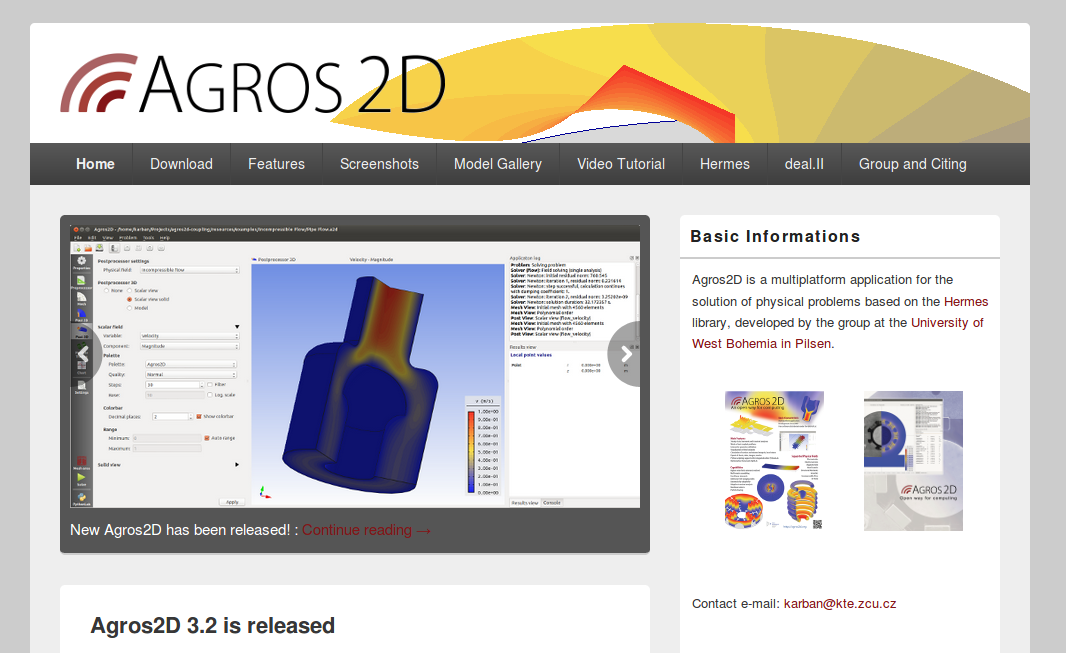
Looking around for open source 2D heat transfer modelling tools I came across Agros2D which is both relatively straightforward to use and from the list of applications and university background evidently very capable.

Website: http://www.agros2d.org/

Installation

Agros2D is available for Linux, Windows and MacOSX. See the Download page for installation details relevant to your operating system.

The suggested installation procedure for Ubuntu Linux is the following. Although Agros2d is also available in the Ubuntu Software Center.

sudo add-apt-repository ppa:pkarban/agros2d
sudo apt-get update
sudo apt-get install agros2d

Getting started

Before exploring a run of different models, comparing 1D results with the results from a 2D simulation. I thought I would start with a brief guide on using Agros2D to show how it works and how to create your own 2d heat transfer simulations. Such as this simple partially insulated wall:

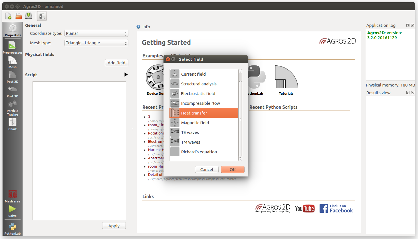
1) Start Agros2D. Click on New and select Heat transfer from the select field list.

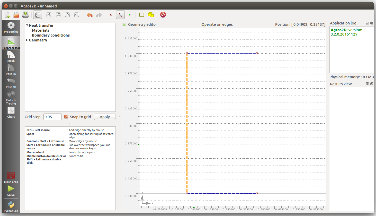
2) Click on the Preprocessor icon in the left-hand menu to open the geometry editor. Click on the red point icon Operate on nodes in the top menu. Hold down the Ctrl key and create a node at position x:0 y:0 with a left mouse click at this position in the geometry editor. Create three more nodes at x:1 y:0, x:1 y:0.5 and x:0 y:0.5 to define a rectangle.

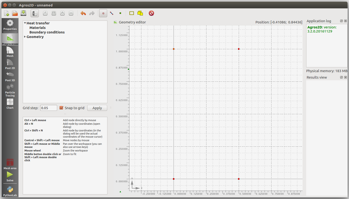
3) Now we will define edges between our nodes. Click on the line icon Operate on edges in the top menu. Hold down the Ctrl key again and click and drag from the first point a line to the next point, repeat to complete the rectangle.

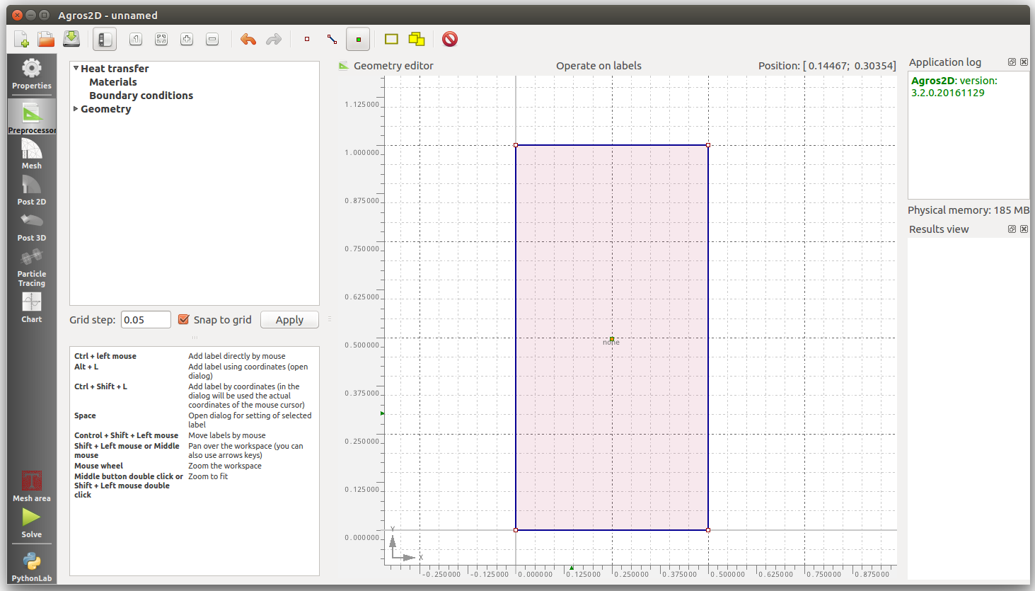
4) The next step is to define a surface. Click on the green point icon Operate on labels in the top menu. Hold down the Ctrl key again and click in the center of the the rectangle to create the label.

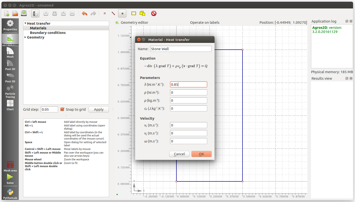
5) Create a material for the element by right-clicking on the Materials title under Heat transfer. Enter an applicable name such as 'Stone Wall' and a thermal conductivity, I have entered 0.85 W/m.K which will result in a wall U-value of 1.7 W/K.m2 for a wall thickness of 0.5m.

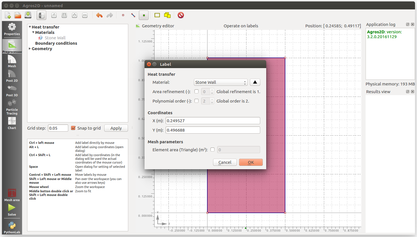
6) To apply the material to the rectangle element first select the rectangle element in Operate on labels mode. Then right-click on the label in the centre of the element and click on Object Properties. Select the Material from the drop down list, click Ok to complete.

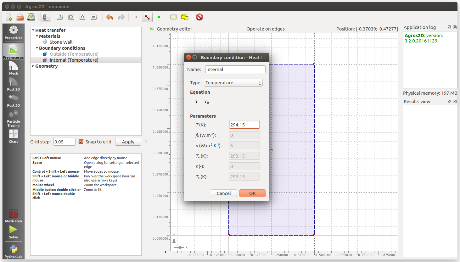
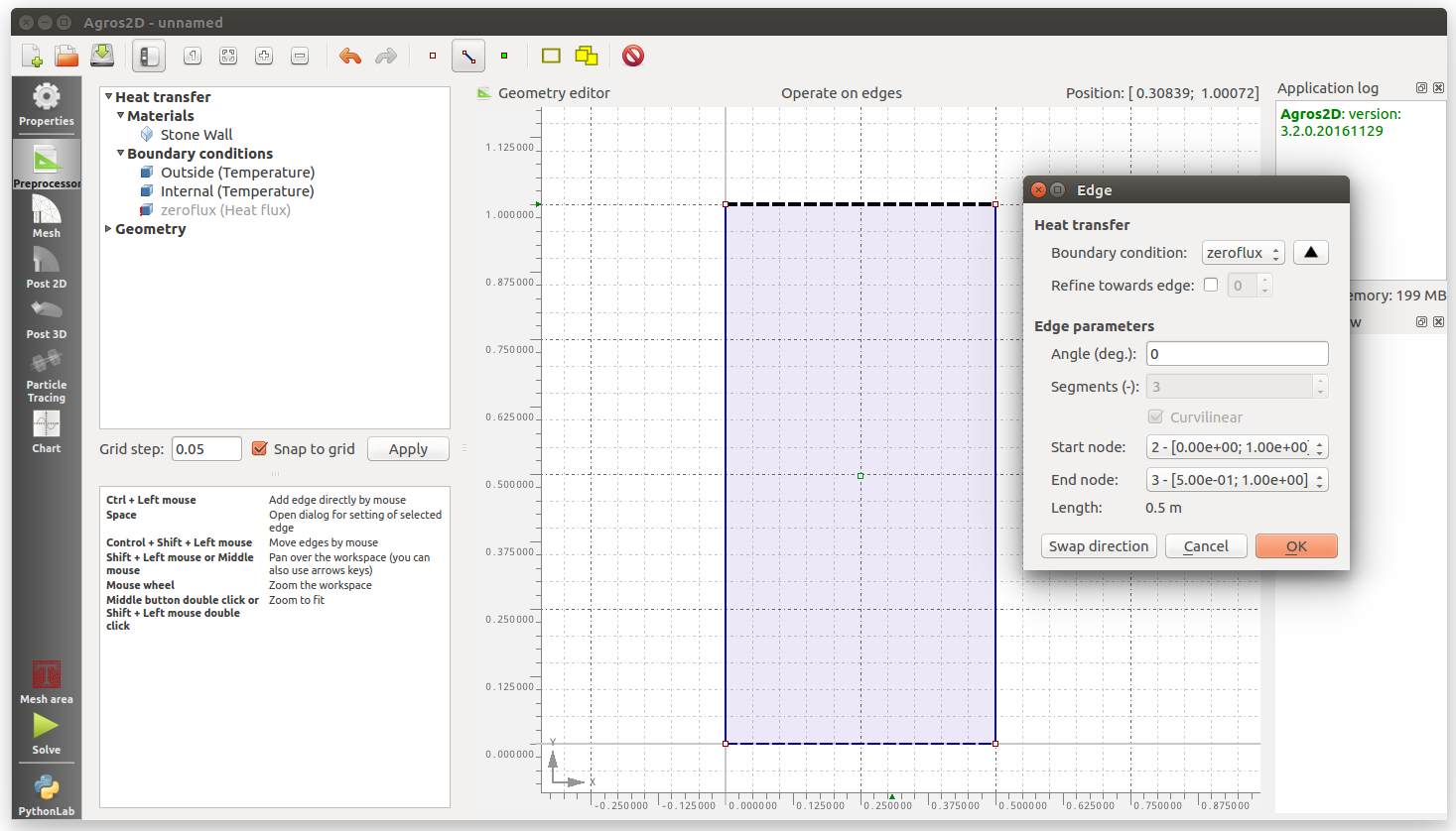
7) The next step is to define boundary conditions for the edges of our element. Boundary condition are used to tell the model that we wish to specify that say one edge of our element is at an outside temperature e.g 10C and another edge is at the internal temperature e.g 21C. It's also possible to define a boundary condition with no heat transfer if we wish to restrict the geometry of our simulation.

Right click on Boundary Conditions and click on New Boundary Condition. Give your boundary a name such as outside or internal, select the temperature type and enter the temperature in Kelvin. 0C is 273.15 Kelvin and so an internal temperature of 21C is 294.15K.

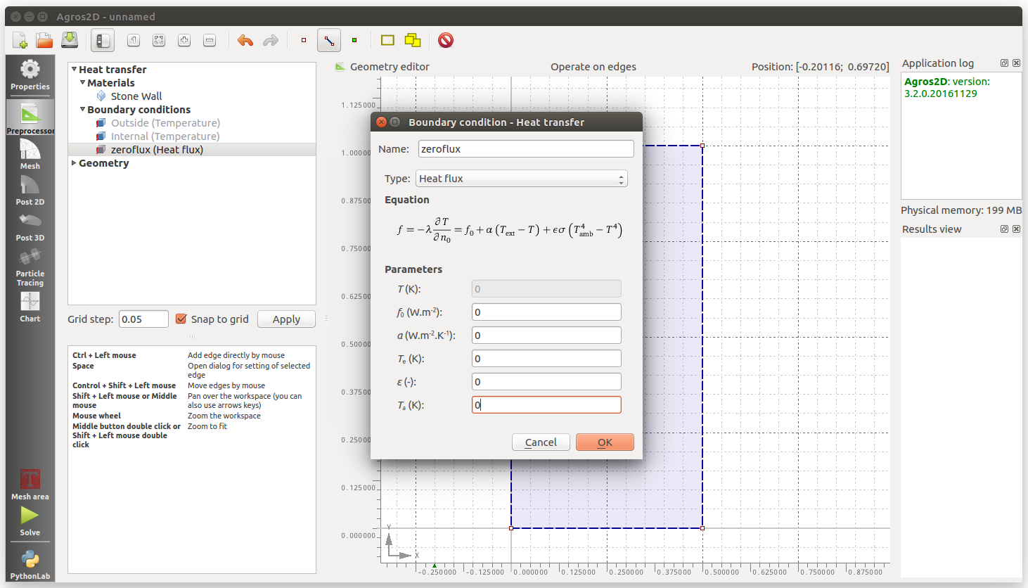
To define an boundary with zero heat flux, select the heat flux type and set all properties to zero.

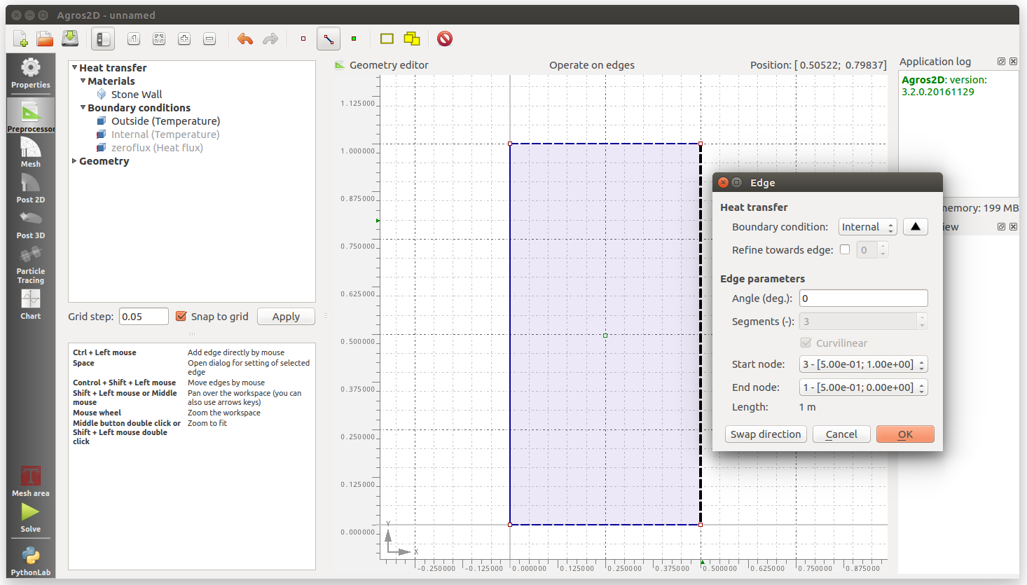
8) To apply a boundary condition select the Operate on edges icon. Select an edge and right click to access object properties. Select the boundary condition from the drop down menu. For this example I have defined the left edge as the Outside temperature boundary condition, the right edge as the Internal temperature and both top and bottom boundary conditions as zero flux. This first example is basically modelling 1D heat transfer but its useful to verify the model results against a basic 1D heat loss calculation.

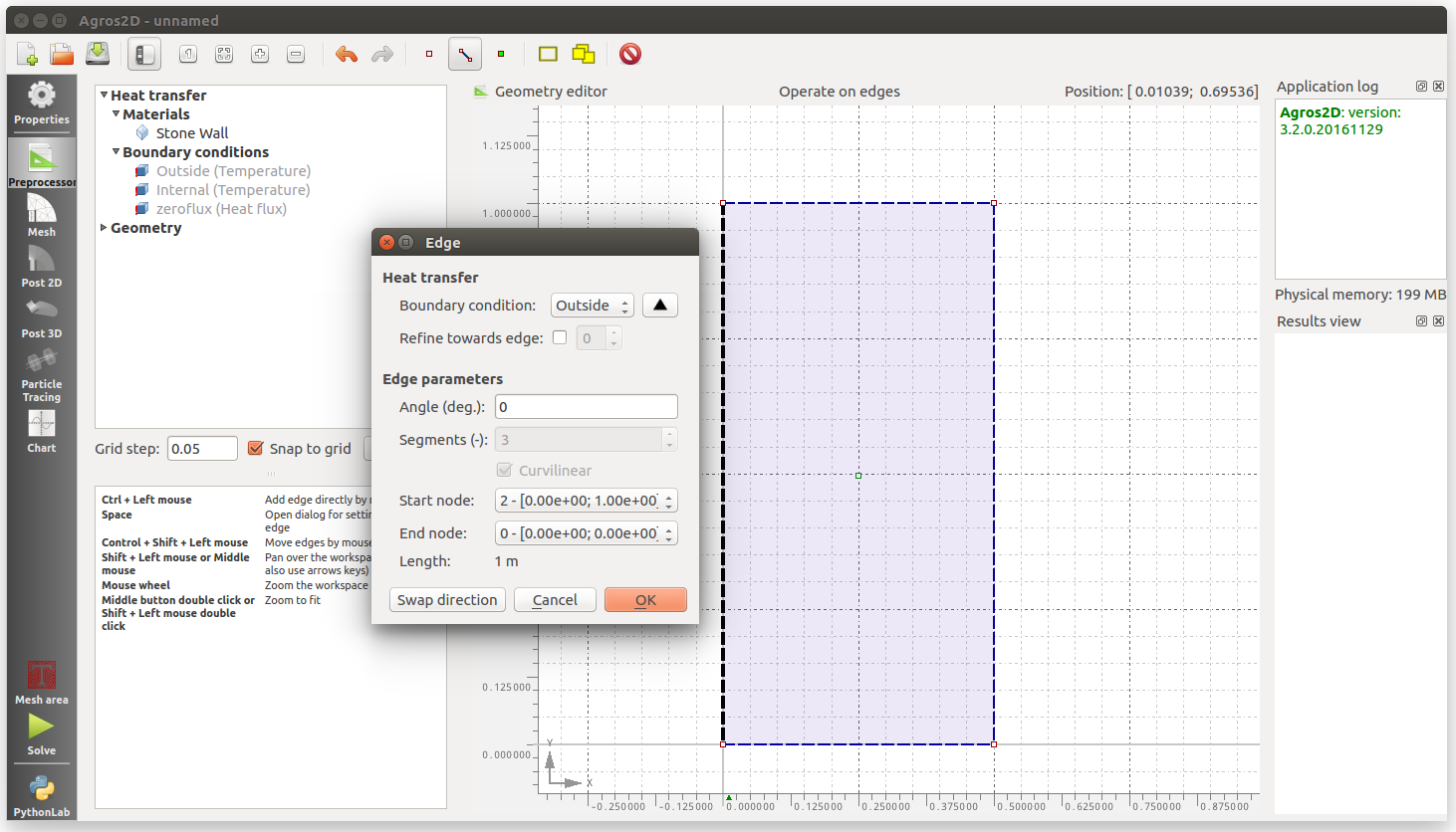
Right edge: Internal temperature boundary condition.

Top and bottom edges: Zero heat flux boundary condition.

9) Finally to run the simulation, click on Solve at the bottom of the left menu:

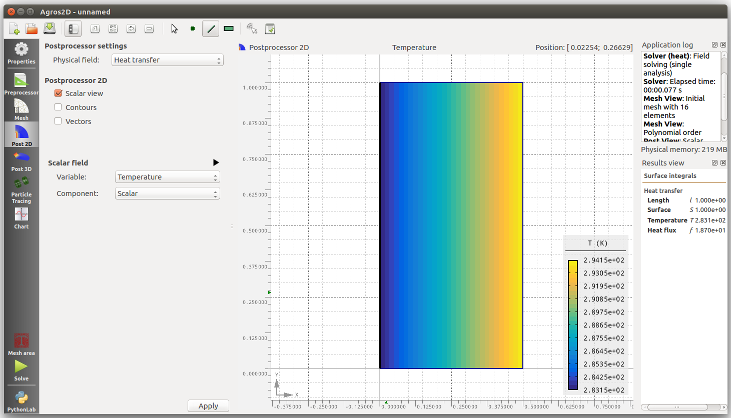
To view the heat loss at the outside edge, select Operate on edges and click on the left side of the element. This will bring up the heat transfer results in the right panel. We can see that the heat flux on the left hand edge here is 1.870e+01 or 18.7 Watts.

We can verify that this is indeed the correct result by calculating the heat loss using the simple steady state 1D equation. (21C-10C) x 1.7 W/K/m2 x 1m2 = 18.7 Watts.

A partially insulated wall

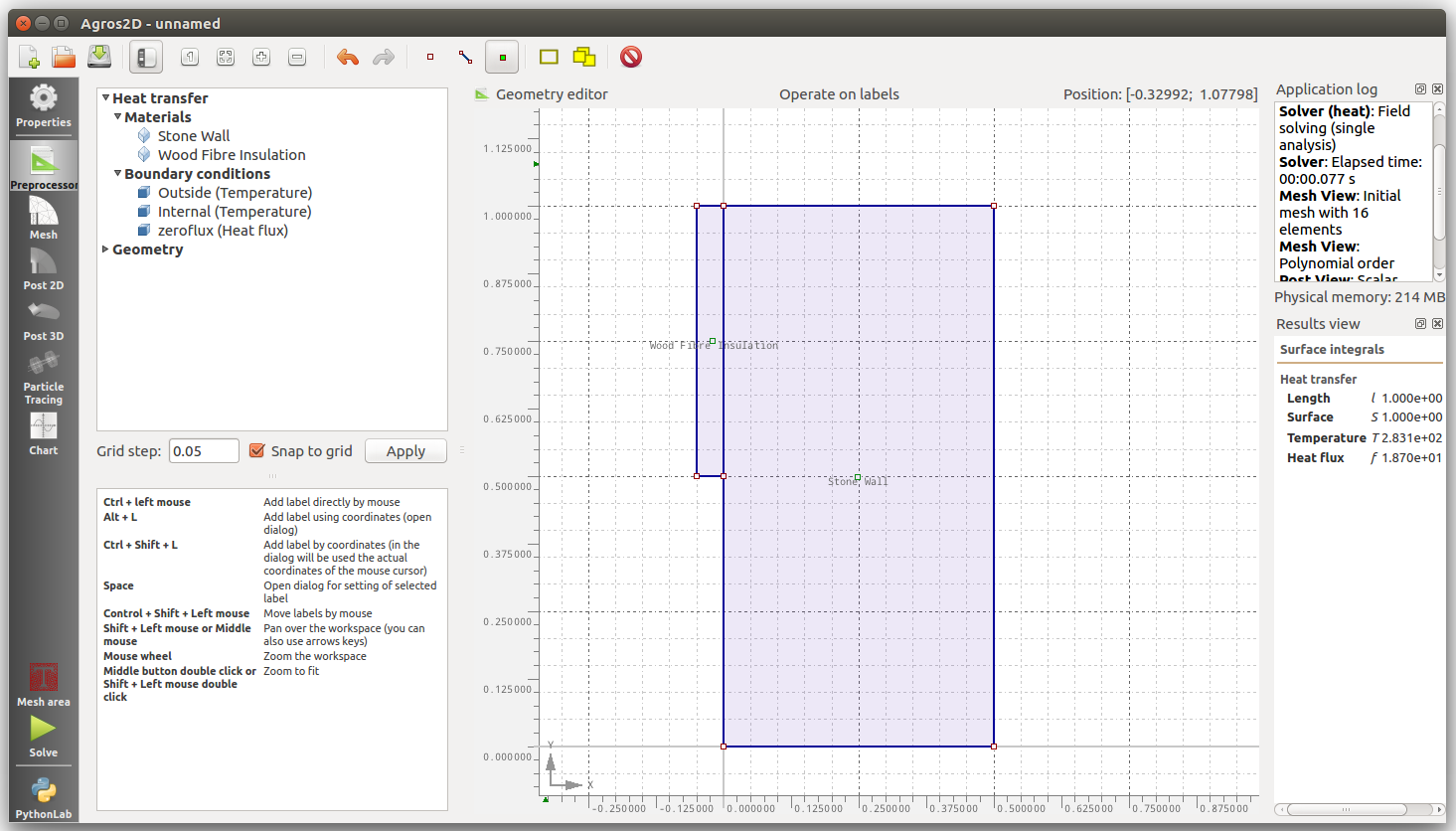
Expanding on the last example a little we can see what happens if we add 50mm of wood fibre insulation to half of our wall element.

1. Delete the stone wall label
2. Delete the left edge
3. Create 3 nodes to define the 50mm insulation layer geometry
4. Join the nodes with edges including an edge between the insulation layer and stone wall
5. Create a wood fibre insulation material with thermal conductivity of 0.39 W/m.K
6. Create a label in the center of the stone wall and define the material as stone wall.
7. Create a label in the center of the insulation layer and define as the wood fibre material.
8. Select the Outside boundary condition for all the externally facing left edges. Select zeroflux for the top edge of the insulation and dont apply a boundary condition inbetween the insulation and stone wall.

The completed geometry:

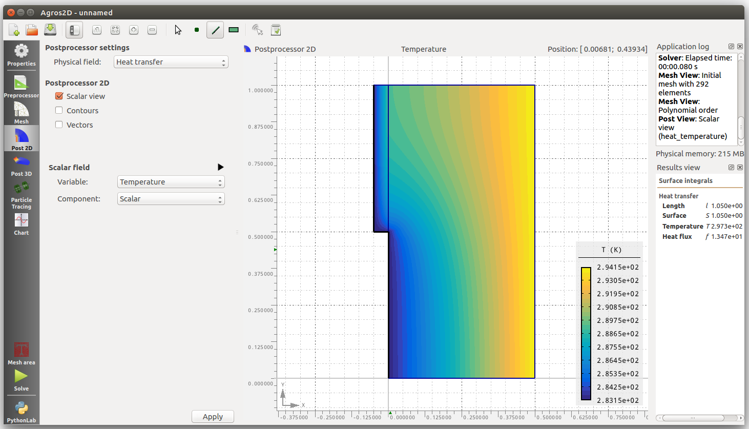
The solved simulation:

Using the edge selector click on each of the outside edges while holding down the Shift key to sum the heat loss across all external edges. We can see that the heat loss is calculated to be 13.47 Watts.

It's important at this point to check that the heat flow into the wall is the same as the heat flow out of the wall. A quick click on the internal edge of the wall shows that this is not the case. The flowing into the wall is 14.5 W indicating a significant error.

We can reduce the error in the simulation by increasing the number of refinements (to ~4) and polynomial order (to ~8) of the mesh which can be set by clicking on the Properties icon in the left menu and then on the Heat transfer icon. I also found the 'Triangle - quad join' mesh type to give a lower error result - however I dont really know enough about the program to comment on what this means. Re-running the solver now takes considerably more time but the heat flow out of the wall becomes much nearer to the heat flow into the wall 14.42W vs 14.46W.

We can now see how a 2D model differs from a 1D calculation.

The U-value of 50mm of wood fibre insulation with a thermal conductivity of 0.39 W/m.K is 0.78 W/K.m2. The combined U-value of the stone wall and 50mm of insulation is 0.53 W/K.m2.

The 1D heat loss through the uninsulated part of the wall is: (21−10)×1.7×0.5 = 9.35 W
The 1D heat loss through insulated part of the wall is: (21−10)×0.53×0.5 = 2.915 W

The sum of this heat loss is 12.265 Watts, 2.155 Watts or 15% less than the more realistic 2D model which illustrates how the higher temperature wall section with the insulation layer looses an amount of heat down and through the uninsulated part.